Introduction to Audio Encoding

In today’s high definition world, we want the best quality in every film, picture, and sound we encounter. Blu-Ray DVD’s seem poised to take over the market, pushing the inferior DVD’s down the same path as the VHS tape. In much the same way, we see digital audio pushing for the same quality. Although the popularity of the iPod and mp3s has given rise to an age of over-compressed, low-quality music, we also see a rise in vinyl sales, as well as developments such as Sony’s Super Audio CD (SACD). This implements a relatively new process to encode audio, paving the way for a massive change in the quality of music we listen to, if it is accepted.

Analog vs. Digital

In order to understand audio encoding, the difference between analog and digital must be understood. Something that is analog is an uninterrupted, pure, natural sound. The human voice, a guitar, and a vinyl record are all examples of analog sound. When a vinyl record is cut, a needle senses the vibrations from an audio source and cuts it exactly into the vinyl. This is why vinyl could be said to have the highest sound quality, and is still popular today, despite many alternatives and developments. An analog signal can encompass all frequencies, even the inaudible. This is why a live orchestra sounds more “full” than a recording, even of the highest quality. Audiophiles will argue that the energy of the inaudible frequencies adds to the quality of sound, even though they cannot be perceived by the ear.

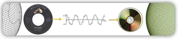A digital signal is a replication of an audio signal by a number of ones and zeros. It is the same way a picture on a computer screen is replicated by thousands of intensity values represented in binary code. The music on an iPod, a compact disc, and an mp3 are examples of digital replication. Even many modern musical instruments have implemented digital sound, from digital keyboards to electronic drums to guitar pedals. Digital sounds can be made with a programmable chip, rather than a circuit, and is much more reliable, inexpensive, and easy to mass produce as a result. However, there are drawbacks to digital sound that sacrifice the sound quality, and these drawbacks are being constantly developed and upgraded to replicate an analog signal more precisely.

Pulse Code Modulation (PCM)

Since the dawn of the compact disc, the method of encoding has been Pulse Code Modulation (PCM). In PCM, the analog signal from a human voice or musical instrument is sampled, or captured, at regular intervals and recreated digitally. This is similar to a flipbook being used to simulate a moving picture. It is not an exact duplication of the audio signal, but it is a close approximation. However, there are two limitations with PCM that prevent it from being the ideal encoding method, despite its longevity in the industry.

Sampling Rate

The first problem with PCM lies in the sample rate. Simply put, this is the number of “snapshots” per second. In a standard audio CD, the sound is sampled 44100 times per second. In mathematical terms, “per second” can be described as Hertz or Hz. So 44100 samples per second can also be stated as 44.1 kiloHertz or kHz.

When referring to the frequency of an audio signal, Hertz is also used. Each note has a distinct frequency, and any instrument can produce a wide range of frequencies. For example, the E string on a bass guitar is approximately 40 Hz, while the highest fret on the G string is around 500–600 Hz. The human ear is capable of hearing in the range of about 20 Hz to about 20,000 Hz. This upper boundary will decrease with age, and with today’s exceptionally loud music, the average person may only hear up to 15,000 Hz. However, this is still a very wide range, and must be accounted for with digital replication.

When an audio signal is sampled, it must follow a rule called the Nyquist Rate. This states that the sampling rate must be at least twice the bandwidth of the audio signal. This means for a 1,000 Hz wave, the sampling rate must be at least 2,000 Hz. Therefore, when sampling an orchestra using all audible frequencies (up to 20,000 Hz), the sampling rate must be at least 40,000 Hz. The decision to make the standard sampling rate 44,100 Hz is explained by early monochrome video recorders. Although the compact disc does not have any video circuitry, the earliest recording processes used the same equipment. There were two different standards for video recording in the 1970's, the PAL and the NTSC, both with different frequencies. 44.1 kHz was simply a compromise between Sony and Philips to achieve global compatibility with audio recording [1].

Thus, 44.1 kHz became the standard sampling rate for audio files. Since it abides by the Nyquist Rate, all audible frequencies can be captured. However, this does not account for the bit depth, which is the other limitation of PCM.

Bit Depth

Bit depth, or quantization level, is basically the number of storage units available for the audio signal to occupy. In binary code, the number of bits is an exponent of the number 2, so a standard 16 bit audio CD would have 2^16 or 65,536 quantization levels. A better example of bit depth is demonstrated in Figure 1.

Here, we see the analog signal, represented by the red line, and the number of quantization levels, represented by the green bars.

In Figure 2, we see the approximation of the analog wave as a digital wave, represented by the blue line.

In this example, there are 10 quantization levels for the signal to occupy. Looking at the analog signal, it is clear that this is not even close to an accurate representation of the signal. As the number of bits are increased, more quantization levels are possible.

Figure 3 shows an audio signal with 40 quantization levels, sampled at a rate of 4 times the sampling rate of Figure 1.

It is evident that increasing the number of quantization levels will increase the quality of the replicated audio signal. However, the standard audio CD is set at 16-bit and 44.1 kHz sampling.

Although compact discs are a lower quality replication than vinyl, they are astronomically better than mp3 files. The bit rate of a compact disc, or the number of bits transferred per second, is about 1,411.2 kilobit/second (16 bit/sample x 44100 samples/second x 2 channels / 1000 bits/kilobit). When decoding to an mp3 file, the number of bits/second is decreased drastically. A standard mp3 will decode at 128 kbit/s. Even the highest quality mp3 will decode up to 320 kbit/s. This is far inferior to an audio CD, which is an approximation of an analog signal in the first place! If new developments in high definition audio are implemented in a resourceful method, the mp3 may not have a very long life span.

1-Bit Modulation

An alternate method of audio encoding has become popular in recent years. The SACD is one example of this, and companies like Sony are marketing home theatre systems with high definition audio in many of their products. The difference between this new, high definition audio and the standard audio in many of today’s products has to do with the way it is encoded. Instead of PCM, a different approach is used called 1-Bit Delta-Sigma encoding.

There are many fundamental differences between 1-Bit sampling and PCM. The method of quantization is the most obvious. In 16-bit PCM, the signal can be captured in as many as 2^16, or 65,536 levels. Although the resolution can be increased by increasing the number of bits, a resistor is needed in the digital-to-analog converter (DAC) for each bit. Therefore, in 16 bit encoding, 16 resistors are needed in parallel to capture the signal. In 32 bit encoding, 32 resistors are needed. Higher resolution means more circuitry, which makes the device more costly.

Direct Stream Digital (DSD)

In 1-Bit sampling, only one quantization level is needed. The signal is read by Direct Stream Digital (DSD) method. This means that instead of looking at the entire amplitude of the signal, only each incoming instant is analyzed consecutively. Each sample has only two reference points, one for increasing amplitude, and one for decreasing amplitude. Hence, using one bit, each instant can be classified as “on” or “off.” Using this method, a staircase-like system of sampling is achieved where each bit reads the analog signal as up or down. This is shown in Figure 4. With DSD, the encoding process will take a much longer time, but the results can be a much higher resolution.

Quantization Noise

Since only one bit is utilized, there is a much bigger chance for “noise” to distort the signal. In digital audio, “noise” is defined as the unwanted information that is a byproduct of recording/sampling techniques. This is commonly seen as “snow” on a television set. In every digital converter, both PCM and 1-Bit, noise is produced in the sampling process called quantization noise. In PCM, there is no way to eliminate this noise. However, 1-bit sampling uses a feedback loop, which compares the output signal to the input signal, to “shape” the noise. Using the feedback loop, we can compare the energy of the input signal to the output signal and eliminate any excess noise that was added in processing. This noise is moved out of the desired signal bandwidth and into very high, inaudible frequencies. Figure 5 shows an example of noise shaping.

Using this feedback loop several times, and comparing several different samples to the original analog sample, the value can be averaged and produce a much higher Signal-to-Noise Ratio (SNR). The number of feedback loops in a 1-Bit encoder is the order of the encoder.

Figure 6 shows the corresponding SNR in dB for different order modulators at various sampling rates.

Oversampling

Notice the Oversampling Rate on the x-axis in Figure 6. This is because a 1-Bit modulator does not sample at 44.1 kHz. Rather, a much higher sampling rate must be used to account for quantization noise. This rate is often 64 times the desired sampling rate, or 64 × 44.1 kHz, or approximately 2.8 GHz! By taking this many samples, the unwanted quantization noise can be shaped for each sample, and the average noise can be much lower. For an Nth order modulator, each time the sampling frequency is doubled, the inband quantization noise decreases by 3 x (2M+1) dB [2]. Doubling the sampling rate for a first order modulator will reduce the quantization noise by 9 dB, but doubling the sampling rate for a second order modulator will reduce the noise by 15 dB, and so forth. This drastically improves the SNR at 64 times the sampling rate. Figure 7 shows the frequency response for the signal and noise of a first and second order modulator.

At low frequencies, noise is suppressed more efficiently with each increase in order. However, due to noise shaping, higher frequencies are often distorted in 1-Bit modulation. This is sometimes preferable to PCM, which has low-level quantization noise across all frequencies.

Decimation

Since the human ear can only detect frequencies up to 20 kHz, a sample rate of 2.8 GHz produces vastly redundant data. To return the signal back to a realistic stream, a process called decimation will return the output to 44.1 kHz. This is done by using every 64th sample. Figure 8 shows a visual example of decimation.

Conclusion

Thus, 1-Bit modulation has been implemented in many new “high definition” audio devices, and developers continue to use this process to expand into multi-bit modulators and other hybrid converters. It has become accepted among audiophiles, and is slowly taking the place of PCM. Is one better than the other? It is still debatable. However, 1-Bit modulation allows for simpler circuitry and much better noise shaping in lower frequency bands. The SNR is much better than PCM, except in the higher frequency range, where much of the noise is inaudible anyway. The design is simpler, using more digital implementation than PCM, and as programming advances, digital functions like noise shaping will be enhanced.

Once 1-Bit modulation starts to become affordable, consumers will begin to realize the poor quality of mp3's. Steps will be made to expand 1-Bit audio into the portable market, and “high definition” audio will become the norm. Until then, only the select few who have heard the differences will know how much better sound quality can be, and will only strive to educate the rest.

References:

[1] John Watkinson, The Art of Digital Audio, 2nd edition, pg. 104[2] James C. Candy, Gabor C. Temes. “Oversampling Methods for A/D D/A Conversion, Oversampling Delta-Sigma Converters, ” New Jersey, IEEE Press, 1992., p. 3–7.

[2] Figures 1,2, & 3 were Adapted from “Why does it say 1-bit Dual D/A converter on my CD player?”. April 23, 2001 http://entertainment.howstuffworks.com/question620.htm (November 12, 2007)

[3] Figure 4. 1-bit sampling of standard sine wave. Adapted from An Introduction to Delta-Sigma Converters, Uwe Beis, August 2007. http://www.beis.de/Elektronik/DeltaSigma/DeltaSigma.html

[4] Figure 5. Noise shaping removes the quantization noise from a Delta-Sigma Modulator. Adapted from “Getting the Most Out of Delta-Sigma Converters, ” Russell Anderson, Analog Zone. http://www.analogzone.com/acqt0310.pdf

[5] Figure 6. Delta Sigma Conversion Noise – SNR vs. Oversampling Rate and Modulator Order (0 – 5). Adapted from An Introduction to Delta Sigma Converters, Uwe Beis, August 2007. http://www.beis.de/Elektronik/DeltaSigma/DeltaSigma.html

[6] Figure 7. Frequency Responses Causing Noise Shaping. Adapted from An Introduction to Delta Sigma Converters, Uwe Beis, August 2007. http://www.beis.de/Elektronik/DeltaSigma/DeltaSigma.html

[7] Figure 8. Decimation in the Time Domain. Adapted from A Brief Introduction to Sigma Delta Conversion, David Jarman, May 1995. http://www.intersil.com/data/an/AN9504.pdf